Building a database II - B-Trees
Explore how B-Trees work, their role in database indexing, and how they compare to LSM trees. This post covers insertion, search, and deletion with a hands-on implementation, highlighting key challenges like restructuring. A great starting point for developers diving into B-Trees! 🚀
Introduction
n a previous post, I implemented a key-value datastore using a Log-Structured Merge (LSM) tree as its backend. This time, I wanted to explore another widely used indexing structure—B-Trees. Given their importance in databases and storage systems, I decided to implement one myself to deepen my understanding. Here’s how it turned out.
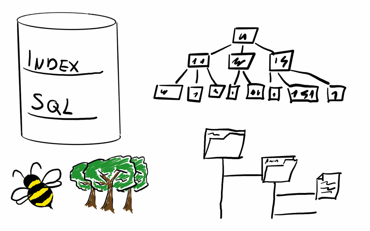
How B-Trees work
B-Trees are fundamental to database indexing and are widely used in relational database management systems (RDBMS) and filesystems. They are self-balancing search trees that generalize binary search trees by allowing each node to have multiple children. This design enables efficient, logarithmic-time operations for searching, inserting, and deleting keys while keeping disk access minimal.
A particularly useful resource I found while implementing my B-Tree was this interactive demo, which visually demonstrates how B-Trees handle insertions and deletions. I used it extensively to test my implementation and compare results.
A B-Tree is defined by 5 properties:
- Every node has at most m children.
- Every node, except for the root and the leaves, has at least ⌈m/2⌉ children.
- The root node has at least two children unless it is a leaf.
- All leaves appear on the same level.
- A non-leaf node with k children contains k−1 keys.
m is called the order of the tree.
B-Trees vs LSM Trees
How log structured merge trees and B-Trees differ?
| Aspect | LSM Trees | B-Trees |
|---|---|---|
| Write Performance | High: Writes are fast due to sequential log appends and batching. | Moderate: Writes are slower due to in-place updates and frequent disk I/O for rebalancing. |
| Read Performance | Moderate to Low: Reads may require checking in-memory store and multiple SSTables on disk. | High: Reads are efficient with a single disk lookup due to the balanced tree structure. |
| Use Cases | High-write workloads: Suitable for write-heavy systems like time-series databases and logging. | General-purpose workloads: Best for balanced read/write operations like file systems and OLTP. |
| Disk Use | Efficient: Compact storage due to log merging and level compaction, but write amplification occurs. | Higher: Requires more disk space due to tree node storage and in-place updates. |
| Memory Use | High: Requires significant memory for write buffers and Bloom filters to optimize reads. | Moderate: Memory use is proportional to the size of internal and leaf nodes. |
| Applications | Cassandra, LevelDB, RocksDB: Used in NoSQL and write-intensive applications. | MySQL, PostgreSQL, NTFS: Common in relational databases and file systems. |
The implementation
Before going into details it is important to mention that with B-Trees it is absolutely possible for different implementations to produce different structures for the same dataset, depending on how they handle insertion, splitting, and balancing. So if the results from my solution does not match your rs some example, it is possible that it is using a different flavor, but by checking the above discussed 5 properties we can always verify if a tree is correct.
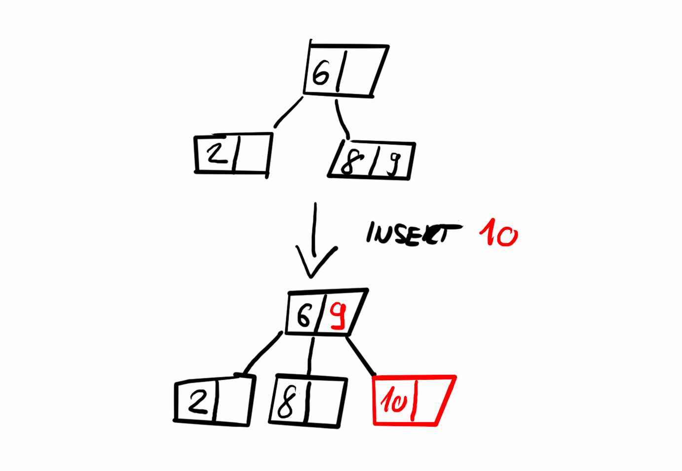
Inserting an item
A new item is always inserted into a leaf node. We start by navigating the tree to locate the appropriate leaf node where the item should be placed. In some cases, inserting an item may require restructuring to maintain the five properties of a B-Tree discussed earlier. The algorithm I used handles this preemptively: while traversing the tree, it splits any full nodes encountered along the way. This ensures that the insertion at the leaf level is possible and prevents a cascade of restructuring from the bottom up.
Splitting a node involves creating a new sibling node and moving half of the keys and children from the full node to the new node. After the split, we determine whether to continue the search with the original node or the new one before making a recursive call.
Searching for an item
Searching in a B-Tree is straightforward. We start at the root node and iterate through its keys. If we find the key we are looking for, the search is complete. Otherwise, we recursively continue searching in the appropriate child node—the one where the key is greater than the key we are searching for. This approach leverages the sorted structure of B-Tree nodes to efficiently guide the search process.
If we reach a leaf node without finding the key, we can conclude that the key does not exist in the tree.
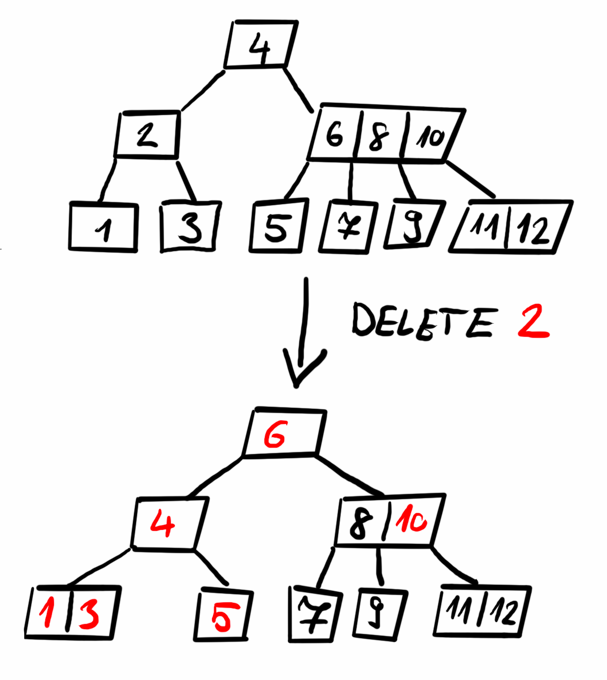
Deleting an item
When deleting a key, three main cases arise:
- If the key is in a leaf node, it is simply removed.
- If the key is in an internal node, it is replaced by its predecessor (largest key in the left subtree, the largest left key) or successor (smallest key in the right subtree, smallest right key). If neither subtree has enough keys, the two children are merged.
- If the key is in a child node with fewer than the minimum required keys, we balance the tree by either borrowing a key from a sibling or merging the node with a sibling. This rebalancing is done preemptively while searching for the key to delete, ensuring that the node we delete from remains compliant with B-Tree properties.
Summary
B-Trees are widely used, and researching their implementation was incredibly interesting. I found them significantly more difficult to understand than LSM trees. The restructuring steps, particularly during deletion, can be quite tricky, but implementing them was a great learning opportunity. My current solution is in-memory only, but B-Trees offer significant advantages when stored on disk—something I may explore further in future iterations.
The code is available on GitHub.
The Wikipedia article is a great source as almost always.