Building a Database III - Bloom filters and performance

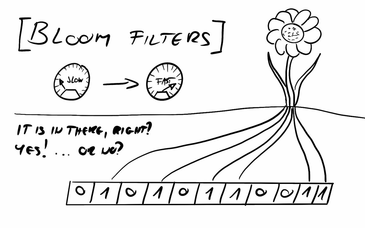
Bloom filters are fascinating data structures that provide a clever way to save both space and time when looking up data in a database. They excel at answering a simple yet powerful question: Is this item in the set? Well… almost.

In this article, I'll take a hands-on approach—after a brief introduction to the concept, I'll dive into how I integrated Bloom filters into my Log-Structured Merge (LSM) Tree-based datastore and implemented key performance optimizations along the way.

Bloom filters

The basics of Bloom filters

Bloom filters are known as probabilistic data structures because they can determine with 100% certainty that an item is not in a set, but they have a small chance of falsely indicating that an item is present when it isn’t. In other words, Bloom filters never produce false negatives, but they can produce false positives.

So where does this behavior come from?

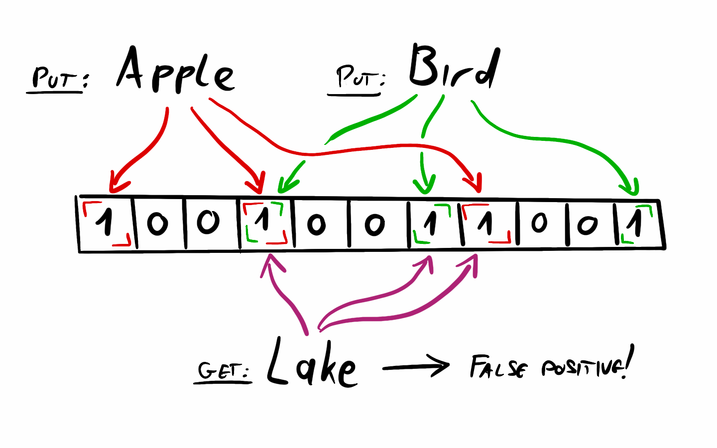
A Bloom filter is simply a fixed-size array of bits (zeroes and ones). It saves space by not storing the actual items. Instead, when inserting an item, the filter hashes it using multiple hash functions. The output of each hash function determines an index in the bit array, and the bits at those positions are set to 1.

When checking if an item is in the set, the Bloom filter applies the same hash functions and checks the corresponding bits. If any of these bits is 0, the item is not in the set—guaranteed. However, if all the bits are 1, the filter assumes the item is present. The catch is that hash collisions can occur, meaning different items might set the same bits. This is why false positives are possible: an item may appear to be in the set simply because other items have set the same bits.

Bloom filters have many use cases. One that I'm going to demonstrate is reducing the number of disk lookups in databases for non existent keys. Others include:

• Checking if a username is already taken
• Filtering malicious URLs, blocked IPs
• Improving cache performance by checking if an URL was visited before at least once already

Tuning the error rate

Bloom filters have parameters we can tune. These are the size of the bit array used for storage, an number of hash functions used. If we know how many items we want to store in the filter (n), and what false positive (p) rate is acceptable we can calculate how many bits and hash functions we need. The equations for this are the following:
m (number of bits needed) = ceil((-n * log(p)) / pow(2, log(2)));
k (number of hash functions needed) = round((m / n) * log(2));

This cool website let's you play around with these numbers and calculate the parameters yourself, but I also built these into my solution.

Bloom filter calculator

Calculate the optimal size for your bloom filter, see how many items a given filter can hold, or just admire the curvy graphs. Also borrow my MIT licensed Javascript for your own programs.

Good to know

Some other interesting facts about Bloom filters include:

• From a basic Bloom filter we can't delete items, however there are counting Bloom filters, where every bit is a counter. When we would set it to 1, we increment it. In case of a deletion the value is decremented. This way we can keep track of how many times a bit was set.
• Bloom filters provide O(k) performance as running the hash functions and accessing an array are all constant time operations.
• A Bloom filter might require numerous hash functions that could be difficult to provide. Often combinations of hash outputs and bit manipulations help create make up the numbers
• The hash functions used don't have to be cryptographic, but should be consistent and give a uniform distribution with efficient computation. MurmurHash3 and similar implementations are often used.

Implementing a Bloom filter in Java

Adding a Bloom filter to the datastore was fairly straightforward. In a Log-Structured Merge Tree (LSM tree), the Bloom filter is the first step in key lookups within an SSTable. Before performing a more expensive search, the filter is checked. If it indicates that the key is not in the SSTable, the search can immediately move on to the next one, avoiding unnecessary disk reads.

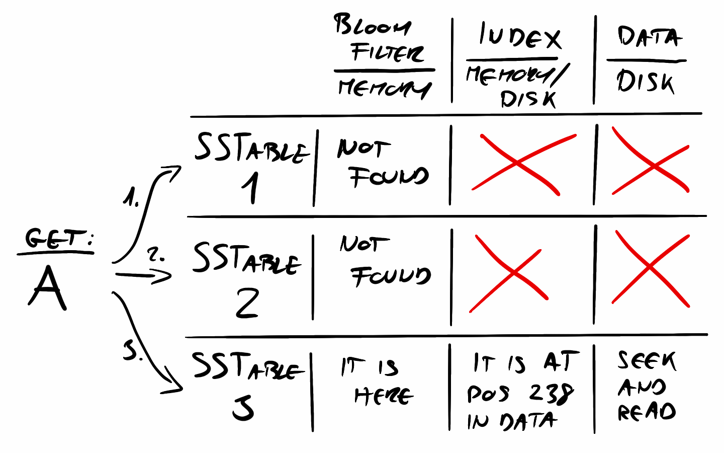
If the Bloom filter indicates that the key might be present, the lookup proceeds as usual—consulting the index to find the key's location and retrieving the value from the data file. However, the Bloom filter significantly speeds up lookups by allowing us to skip both the index and data file checks when we know the key isn’t there.

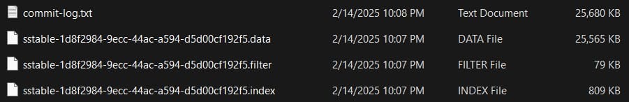
In a typical SSTable setup, there are three main data structures:

1. The data file, which stores the actual key-value pairs.
2. The index, which maps keys to their positions in the data file (typically 1–5% of the data size).
3. The Bloom filter, which acts as a fast, in-memory check (0.1–1% of the data size).

Since the data and index are usually stored on disk, lookups can be expensive. But because the Bloom filter is small enough to fit in memory, it helps eliminate unnecessary disk reads, making key lookups much faster.

So, I knew where to put the Bloom filter in my code, but how should I implement it? The first step was choosing a hash function. My research showed that MurmurHash3 is commonly used, and I found that I could apply bit manipulation to its output to simulate multiple hash functions from a single one.

Since implementing a hash function from scratch wasn’t my main focus, I decided to use the implementation from Apache Commons, which already provides MurmurHash3.

public class MurmurHashFunction implements HashFunction {
    @Override
    public int hash(byte[] input) {
        return MurmurHash3.hash32x86(input);
    }
}

As for the actual Bloom filter, I chose the Java BitSet to store the bits as I found this the most convenient, that let me focus on the logic rather than bit manipulations. BitSet has a variable size, but I tied it to the size of the SSTable so it should never grow larger anyway. I implemented the above mentioned methods to calculate the number of bits and hash functions needed for the requirements.

    private int calculateSize(int expectedElements, double falsePositiveRate) {
        return (int) Math.ceil(-expectedElements * Math.log(falsePositiveRate) / (Math.log(2) * Math.log(2)));
    }

    private int calculateHashFunctions(int expectedElements, int size) {
        return (int) Math.round((size / (double) expectedElements) * Math.log(2));
    }

The most interesting part is how the hash functions are used with add and isPresent.

    public void add(K key) {
        processKeyHashes(key, bitSet::set);
    }

    public boolean isPresent(K key) {
        return processKeyHashes(key, index -> {
            if (!bitSet.get(index)) {
                throw new RuntimeException("Not present");
            }
        });
    }

    private boolean processKeyHashes(K key, Consumer<Integer> indexProcessor) {
        int hash1 = hashFunction.hash(key.toString().getBytes());
        int hash2 = (hash1 >>> 16) | (hash1 << 16); // Mix bits for variation

        for (int i = 0; i < hashFunctions; i++) {
            int hash = (hash1 + i * hash2) & Integer.MAX_VALUE;
            int index = hash % size;
            try {
                indexProcessor.accept(index);
            } catch (RuntimeException e) {
                return false;
            }
        }
        return true;
    }

Both add and isPresent apply the same hashing logic, which I implemented using a functional Consumer parameter. The hashing itself uses double hashing to generate multiple hash values from a single hash function.

I also made the Bloom filter serializable to disk, similar to the index file. Additionally, I refactored the serialization and deserialization process for both of these files, improving the overall organization. Now, both BloomFilter and Index are more autonomous and encapsulated, making them independent from SSTable.

Integrating the filter into the SSTable was straightforward. Aside from instantiating it, the main change was adding a filter check at the beginning of the getValue method.

    public Optional<V> getValue(K key) throws IOException {
        if (!filter.isPresent(key)) {
            return Optional.empty();
        }

        ...

And that is it about implementing the filter and integrating it to the existing codebase.

Tuning the performance

When I finished the filter, I wanted to test its performance because I was really curious about any visible effects. The theory is clear and makes sense—actual databases use very similar mechanisms—so I should see a difference for sure.

I didn’t—and I also ran into some issues.

The test case I wrote creates 400,000 data records with a memtable size of 50,000 records (SSTables have the same size). I wrote two functions to test the put and get performance of my LSM datastore, with and without the Bloom filter. For the tests without it, I just commented out the three lines at the top of the get method in SSTable where the filter is used. The test cases run the tests five times and average out the results.

The data insertion test ran okay, but surprisingly slowly—it took about 63 seconds to insert the 400,000 records. That’s about 6,349.2 records/sec. It was slow but not too suspicious; I didn’t have a baseline and didn’t know what to expect. Then I tried to run the read test, and it just ran and ran with no end.

This is when I checked it using a profiler (VisualVM). The line where the code spent most of its time was this:

Optional<String> firstLineAfterOffset = lines.skip(offset).findFirst();

After reading the docs I quickly realized that this line, called in an iteration to insert the data records line by line into the data file actually has to open the file and iterate through the lines to the offset to read, it is not random access and this iteration over the lines takes a lot of time.

However, there is a class that does exactly what I needed—it lets you skip to an offset right away, like indexing an array, and read from there. It’s called RandomAccessFile. With this class, you can open a file and randomly seek to a specific location using a byte offset parameter.

try (RandomAccessFile raf = new RandomAccessFile(dataFile.toFile(), "r")) {
  raf.seek(offset);
  String result = raf.readLine();

  ...

The only issue with this was that the offset I calculated and stored in the index was a line number, as in my data file every key is on its own line, and storing the line number was logical and the easiest to understand and follow. However, I decided that I needed this fix, as the system wasn’t technically working with any larger dataset. So, I replaced the line number offset with a byte offset, incrementing it by the length of each inserted line in bytes.

After implementing this fix, the code started to work. It managed to do the 100 000 lookups from 400 000 inserted elements in 57.2 seconds on average (with Bloom filter).

This improvement motivated me to look into the write performance as well. Turns out that using the good old BufferedWriter is way more efficient than just calling Files.write all the time creating an open file -> write -> close file loop.

try (BufferedWriter writer = Files.newBufferedWriter(dataFile, StandardOpenOption.CREATE, StandardOpenOption.TRUNCATE_EXISTING)) {
  long offset = 0;

  for (Map.Entry<K, V> entry : sortedData.entrySet()) {
    String line = keySerDe.serialize(entry.getKey()) + SEPARATOR + valueSerDe.serialize(entry.getValue()) + System.lineSeparator();
    writer.write(line);

    filter.add(entry.getKey());
    index.add(entry.getKey(), offset);

    offset += line.getBytes(StandardCharsets.UTF_8).length;
  }
}

The write performance after this change increased to 9975 record / sec, as it took 40.1 seconds to insert 400 000 records. This is about a 35% improvement on write speed.

Write performance is better than read performance, which is consistent with the properties of a Log-Structured Merge Tree. I'm confident that performance can be improved further, and I may explore that in the future, as this optimization has really intrigued me.

But what about the Bloom filter? What happens if I disable it? Interestingly, performance actually improved without the filter. Instead of 57.2 seconds, it averaged 55.6 seconds. While the difference is small, it was consistently better. I believe this is because my index files were already in memory during the reads. In this case, checking the Bloom filter added unnecessary overhead, as looking up the key in the in-memory index was already very fast. In a real-world scenario with larger tables, where the indexes aren't entirely in memory, I’m confident the filters would offer a performance gain by reducing disk access. However, I wasn't able to replicate this use case in my tests. In my current implementation, while the index is persisted to disk, it is always kept in memory while the datastore is running. I didn't want to modify this logic just for this experiment.

Summary

I found Bloom filters to be a very clever concept, and it was both interesting and rewarding to implement one myself. Integrating it into my LSM implementation was particularly satisfying, as it felt like a key missing component in a Log-Structured Merge Tree. However, I’m not entirely happy that the filter didn’t provide any noticeable performance benefit in my system. I may revisit the code and test cases in the future to see if I can make it work as expected. On the positive side, I learned valuable lessons about file read and write performance during my tests and managed to make some meaningful improvements.

My goal with this repository is to keep it simple and use it for experimentation and demonstration, rather than as a high-performance production ready solution. While it’s not meant to be a full-fledged database, now that I’ve covered the more fundamental topics, I may gradually start refactoring it to enhance performance and bring it closer to a more usable datastore.

The code for this article is available on GitHub.